Weak significance is significantly weaker than you think

You may know that $p=.04$ doesn’t mean there’s a $96\%$ chance the effect you’re estimating is real. But that raises the question… What does it mean? Perhaps you can rattle off the textbook definition, but I want to ask a deeper question: What do statistical results with $p$-values in the range near $.05$ actually mean and how much confidence should you place in findings with results in the range of $p=.01-0.10$?

One way to make statistical testing precise is to ask how often a testing procedure gets things wrong. The classical Neyman-Pearson framework does this by relating false-positive rates ($\alpha$), false-negative rates ($\beta$), effect sizes ($\delta$), and sample sizes ($n$). The standard setup you learn in statistics class is to design a study that detects an effect of a given size $80\%$ of the time, while reporting a positive result no more than $5\%$ of the time when there is no effect.

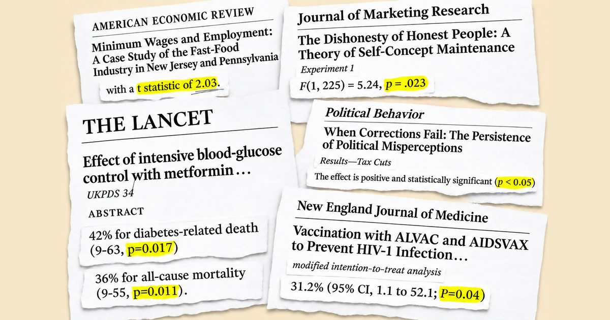
These are useful guarantees, but the Neyman-Pearson framework can only provide them in the “frequentist” sense: they describe error rates across repeated studies.11There’s also a practical challenge: planning for a chosen power requires specifying an effect size to detect and a sample size that can detect it reliably. A defensible target effect can be hard to choose, and with existing or archival data, the sample size may already be fixed. They do not tell us the probability that a particular conclusion is correct. And yet, after running a study, an analyst will naturally want to ask: Given what I observed, how likely is it that the effect is real? The Neyman-Pearson approach does not directly answer that question in any meaningful sense. Despite this limitation and repeated warnings against relying solely on $p$-values and significance thresholds (Wasserstein & Lazar, 2016), researchers across many fields still interpret evidence differently depending on which side of $p=.05$ a result falls — even researchers with PhDs and graduate statistical training (McShane & Gal, 2016, 2017).

So rather than asking everyone to change how they conduct statistical tests, I want to offer a perspective on the $p$-values we are all already familiar with that attempts to make their weaknesses quantifiable and apparent. In particular, I will focus on demonstrating why $p$-values in the range of $p=.01-0.10$ provide much weaker evidence than is implied by how often these quantities are used as decision criteria.

Interpreting weakly significant $p$-values with very few assumptions

Consider that if you are conducting any statistical analysis, you are almost by definition walking into that analysis with some non-zero belief that the null hypothesis is true and some non-zero belief that the null hypothesis is false. If you knew already that $\text{Pr}(H_0)=0$ or $\text{Pr}(H_0)=1$, why would you need statistics?

Let’s call this starting probability $q$: how likely you thought a real effect was before seeing the result. Here, “no effect” means exactly zero effect on the quantity being tested. In mathematical terms, $H_0:\delta=0$, $H_1:\delta\neq0$, and $q=\Pr(H_1)$.

In Bayesian terms, $q$ would properly be called our “prior” belief about the existence of a real effect. You may reasonably object that you don’t have a precise number in mind, or that you are not comfortable inserting your personal belief into a statistical analysis.22There are structured methods for eliciting informed judgments (O’Hagan, 2019), as well as empirical methods for estimating the proportion of real effects from collections of related tests (Storey, 2002), that may be suitable depending on your study’s context. That’s fine; for now, I just want to make this starting assumption explicit. In doing so, we will be able to build some intuition about how different values of $q$ affect what will be a Bayesian interpretation of $p$-values. However, I will also discuss how this analysis remains informative for how we interpret $p$-values even if you bring no prior estimate for $q$.

In Bayesian analysis, we update our beliefs using the observed evidence. Here, our initial beliefs are quantified as $q=\Pr(H_1)$ and our primary quantity of interest will be our posterior probability of a real effect, which we’ll call $q_{\text{post}}=\Pr(H_1\mid P=p)$: the probability of a real effect after observing the $p$-value.

Before proceeding, note that $q_{\text{post}}$ is exactly the quantity we all wish $p$-values actually represented: the probability of an effect size being real! Assuming we can estimate $q_{\text{post}}$, we can read it as a direct probability whether or not an effect exists.

The catch is that our starting belief and a $p$-value aren’t enough to tell us exactly how convinced we should be. We’d normally need to say more about the effect itself: how large it might be and what results we’d expect if it were real.

However, a useful insight can be found in an underappreciated 2001 paper by Sellke, Bayarri & Berger (SBB), Calibration of p Values for Testing Precise Null Hypotheses. Rather than asking ‘What is the probability that the effect is real?’, the authors ask a simpler question: how strong could the evidence from a given $p$-value possibly be? Across a broad class of models for real effects, they derive a limit on how much an observed $p$-value can favor an effect over no effect.33The calibration applies across a broad class of models used in comparisons of means, $t$-tests, linear regression, logistic regression, Poisson regression, and A/B tests. These are everyday tools across medicine, economics, psychology, and empirical science. (Mathematical details in technical notes)

The fact that we are just considering a bound on the largest possible posterior update makes this approach incredibly powerful: it remains valid without having to specify an effect size, choose a distribution of possible effects, or supply the sample size separately. The calculation needs just two inputs: your starting probability $q$ and the observed $p$-value. What we get is a ceiling on the probability of a real effect using the evidence in the observed $p$-value.

The widget below calculates the SBB bound on increases in the probability of a real effect. The way you should think about this is as follows:

• Start with how likely you thought an effect was ($q=\text{Pr}(H_1)$) and your statistical test’s $p$-value.
• The widget shows how much your beliefs would change in the scenario that is most favorable to the statistical evidence compatible with your $p$-value that is mathematically possible.
• This is not a prescription of how much you should update your beliefs; merely an upper bound on how much any given $p$-value can increase posterior belief in $H_1$.

To take a concrete example of how to read the widget: Suppose you initially give an idea a one-in-five chance of having an effect, i.e., $q=20\%$. If you run a study and the result returns $p=.04$, the SBB analysis demonstrates you should have no more than $\mathbf{41.7\%}$ confidence that the effect is real.

The point doesn’t depend on starting out especially skeptical. Suppose you initially thought an effect and no effect were equally likely: $q=.50$. A result of $p=.05$ then supports at most $71.1\%$ confidence in a real effect, leaving at least $28.9\%$ probability of no effect. Even with that starting belief, crossing the significance threshold leaves substantial room for doubt.

What if you don’t want to specify a prior on $q$?

As the widget demonstrates, the results of this approach to interpreting $p$-values clearly depend on the $q$ you start with. Fortunately, there are several ways we can deal with this dependence.

One Bayesian option is to give $q$ a distribution of its own, such as a beta distribution on $[0,1]$, rather than choose a single value.44In this framework, a uniform prior over $q$ on $[0,1]$ gives the same ceiling on effect probability as setting $q=.50$ in the widget. The widget doesn’t show how the distribution over $q$ itself changes, which a fuller Bayesian analysis could explore. Calculation details. But we can also avoid choosing $q$ at all by asking: what is the largest increase in confidence a $p$-value could support, across all starting probabilities? If you have played around with the widget above, you may notice that the size of the update (green arrow) for different $p$-values varies across $q$, but has a maximum value across the whole interval.

The chart below plots this maximum possible update for each $p$-value, maximizing over all starting probabilities $q$.55Writing $U(p,q)$ for the widget’s probability ceiling, the chart plots $\displaystyle \begin{gathered}M(p)=\max_{0\le q\le1}\bigl[U(p,q)-q\bigr].\end{gathered}$ Note this does not tell us anything about what our maximum posterior belief in a real effect should be; it merely says, no matter your prior belief $q$, the observed $p$-value ($x$-axis) cannot increase that prior belief by more than the value on the $y$-axis.

Whatever your starting belief about the presence of an effect ($q=\text{Pr}(H_1)$), a $p=.05$ result can increase that belief by no more than about $22$ percentage points.

What this analysis can and can’t tell us

Keep in mind the widget gives an upper bound on the probability of a real effect and a complementary lower bound on the probability of no effect. The values in the second figure are upper bounds on how much your prior belief can increase in response to evidence in the form of a $p$-value. Because these are bounds, neither of these approaches tells you precisely how much to update beliefs after seeing a $p$-value. This means that this framework should primarily be used to rule out overly confident interpretations of weakly significant $p$-values, rather than as a prescription about how to interpret all $p$-values.

Indeed, the SBB bounds actually have little to say about $p$-values on the order of .001 and smaller. If we set $q=.20$ and observe $p=.001$, the SBB ceiling on the posterior probability of a real effect rises to $93\%$ — this establishes an upper limit without telling us where below that ceiling the posterior probability falls. A different analysis is needed to say how convincing the observed result actually is with any precision. As such, the SBB ceiling is just not all that informative for small $p$-values.

To put it another way: The low posterior belief ceilings seen on large $p$-values ($p \geq .01$) rule out high confidence in $H_1$; the high ceilings observed for very small $p$-values leave open the question of how much confidence you should have in $H_1$.

How convincing is “significance”, really?

This framework allows us to concretely quantify the gap between “statistically significant” and “convincing”. Rather than forcing us to keep the technical definition of a $p$-value in mind, we directly bound the quantity nearly all decision makers actually care about: the probability of an effect being real. This approach applies across a broad class of common statistical models, all without having to specify an effect size, a sample size, or a distribution of possible effects.

With this in mind, think about a study reporting that a policy increases employment, a treatment reduces mortality, or an intervention changes people’s behavior. Suppose that, given your starting belief, even the strongest interpretation of its $p$-value could support at most $60\%$ or $70\%$ confidence that the effect is real.66For example, $q=.30$ and $p=.03$ give an SBB ceiling of $60.0\%$. With $q=.50$ and $p=.05$, the ceiling is $71.1\%$ — roughly $70\%$. These are upper limits on the posterior probability of a nonzero effect, not estimates of that probability. Would you describe the finding differently? Would you repeat it as established fact? Would it change your decision making before building a policy, a medical treatment recommendation, or a scientific theory around it?

I’m not saying all analyses need to demand smaller $p$-values; limited evidence can still be worth acting on. (The level of evidence needed depends on the stakes.) But “statistically significant” can sound a lot more convincing than “at most $\mathbf{70\%}$ confidence under the most generous mathematically plausible interpretation of the evidence”. It is worth keeping this gap in mind when interpreting statistical analyses — or reporting our own.