A Tale of Math & Art: Creating the Fourier Series Harmonic Circles Visualization
I have a friend who describes himself as a recovering pure mathematician. As someone who majored in math in college but has since gravitated toward more applied, number-crunching pursuits, I’ve always liked this description. Despite my best intentions to stave off my cravings, this post is going to be a major relapse.
The venerable 3Blue1Brown YouTube channel came out with a fantastic video on Fourier transforms a few weeks ago. Not long after, I came across this very cool gif of Vermeer’s “Girl with the Pearl Earring”, which uses a clever visualization of Fourier approximations to “draw” the image with a series of animated, concatenated circles.
Generative Art. pic.twitter.com/5dW7uvDqHR
— じゃがりきん (@jagarikin) February 10, 2018
I could not track the source of the image down, but—with the 3Blue1Brown video fresh in my mind—I was thoroughly determined to understand the math behind this visualization. I took Fourier Analysis as a sophomore in college, but it has been quite a while since I really grokked it.
This led me on down the foolhardy path of recreating this visualization myself. It turns out the math behind this visualization isn’t completely incomprehensible. (The animation/visualization, on the other hand, is an entirely different story.) Rather than going over all the details of the math/code behind the visualization, I will instead use the post as an opportunity to provide some intuition as to how something this cool is even possible. We’ll be taking some pretty big leaps through a good deal of math, but hopefully this will leave you with some intuition for how you might be able to get from a basic understanding of linear algebra and calculus to the math behind the visualization.
A Crash Course in Fourier Analysis
As opposed to taking an engineer’s approach to the problem (which may have more practical value), I like to motivate Fourier analysis using linear algebra (which, as would be expected from a math major, is more elegant).
Let’s start by revisiting vector spaces. Note how vectors in 3-dimensional euclidean space can be represented as the sum of three basis vectors: the point \((3,7,1)\) can be written as \(3e_1 + 7e_2 + 1e_3\), where \(e_k\) represent the “canonical” basis vectors of \(\mathbb{R}^3\):
\[e_1 = (1,0,0)\] \[e_2 = (0,1,0)\] \[e_3 = (0,0,1)\]The key idea behind Fourier approximations is to think of functions themselves as vectors in some infinite-dimensional vector space. This seems weird at first, but it’s not as far out as it may seem. The key to understanding a vector space is to identify a basis of that space (this is essentially what linear algebra is all about). So what would a basis for the infinite-dimensional vector space of functions look like? If you’ve taken a college calculus course, then you’ve likely already found at least one solution to this problem in the form of Taylor series expansions.
Note how the Taylor series of a function allows us to represent any function as an infinite sum of some set of coefficients times the monomials \(t^n\):
\[f(t) = \sum_{n=0}^\infty \frac{f^{(n)}(0)}{n!} t^n\]In terms of linear algebra, this means that the set of monomial powers \(\{ t^n : n \in \mathbb{N} \}\) forms a basis over the infinite-dimensional space of continuous single-variable functions.
This brings us to one of the main ideas behind Fourier series: the set of functions \(\sin(nt)\) and \(\cos(nt)\) (for \(n \in \mathbb{N}\)) forms an orthonormal basis for periodic functions (to be pedantic, I must add “with respect to the inner-product defined by integration over \([-\pi, \pi]\)”). I won’t get too far afield by discussing inner-product spaces and orthogonal functions (this seems to be a decent overview), but I just want to point out the fundamental similarities between thinking of functions as linear expansions over the monomial basis and the Fourier basis.
The unintuitive and surprising aspect of Fourier series is that the set of sine and cosine functions with integer frequencies actually can span the whole space of arbitrary single-variable functions. But—if we can take this for granted—the fact that we can express an arbitrary function as an infinite sum in some basis for this space actually isn’t that crazy. In terms of math, this can be restated by saying there exists a set of coefficients \(a_n\) and \(b_n\) for which the following equation holds for all \(t\) in a given interval \([-T, T]\):
\[f(t) = \sum_{n=0}^\infty a_n \cos(2\pi nt/T) + b_n \sin(2\pi nt/T)\]Crazy Math to Pretty Circles
I won’t get into the full relationship between Fourier series and Fourier transforms (that’s what Wikipedia is for after all), but whenever you see sines and cosines in analysis, you can expect to find some relationship to Euler’s formula lurking around the corner. And whenever you see Euler’s formula, you should expect a very close connection to circles in the complex plane. This is indeed the case with Fourier series and is at the heart of the visualization above. In short, the Fourier expansion of a single-variable real-valued function can be thought of as the real component of a more generalized expansion that makes use of Euler’s formula:
\[f(t)=\sum_{n=-\infty}^\infty c_n\, e^{2\pi i\left(\frac{n}{T}\right) t}\] \[= \sum_{n=-\infty}^\infty \left( a_n - i b_n \right) \left( \cos(2\pi nt/T) + i \sin(2\pi nt/T) \right)\] \[= \sum_{n=-\infty}^\infty {\Large[} a_n \cos( 2\pi nt/T ) + b_n \sin( 2\pi nt/T ) {\Large]}\] \[+ i {\Large[} a_n \sin( 2\pi nt/T ) - b_n \cos( 2\pi nt/T ) {\Large]}\]In this last formula, you can see the similarity between the real component of the function and the Fourier series expansion mentioned above. (If you click through to the Wikipedia article, you’ll see that the \(c_n\) coefficients are directly computable from the Fourier transform of the given function \(f\).)
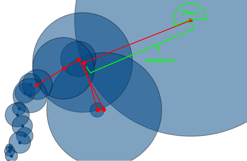
Once we have these pieces in place, it’s not too much of a jump to generate the spinning circles visualization. Euler’s formula is the real star here, which allows us to cleanly decompose each point in the complex plane into an angle (the argument to the exponential function) and an amplitude (the \(c_n\) coefficients). If you think about how to visualize the sum of many points in the language of angles/amplitudes for long enough, you’ll find a direct connection to imagining each term in the infinite series above as representing a point on a circle with radius \(c_n\), offset by \(2\pi nt/T\) radians.
The image below demonstrates how a simple sum of complex numbers in terms of phases/amplitudes can be nicely visualized as a set of concatenated circles in the complex plane. Each red line is a vector representing the a term in the sequence of summands: \(c_n e^{2\pi i\left(\frac{n}{T}\right) t}\). Adding the summands corresponds to simply concatenating each of these red vectors in complex space:

Pretty Circles to Animated Drawing
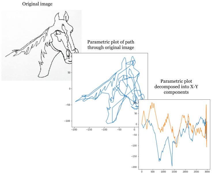
With all the abstract mathematical pieces in place, it’s not too much more work to arrive at a fully animated visualization. If you have a line drawing in 2-dimensional (x-y) space, you can describe this path mathematically as a parametric function, which is essentially just two separate single variable functions, both in terms of an auxiliary variable (\(t\) in this case):
\[f(t) = ( x(t), y(t) )\]Below, I’ve taken a simple line drawing of a horse, found a (crudely-derived) parametric path through the black pixels in that image, and seperated that path into its X and Y components.

At this point, we need to calculate the Fourier approximations of these two paths, and use coefficients from this approximation to determine the phase and amplitudes of the circles needed for the final visualization. This post is mainly meant to be a light introduction to the underlying concepts behind this visualization, so for any more of the specific implementation details on how to create the animation, I am going to defer to the corresponding Jupyter notebook for this post. You can find the static (browsable and downloadable) notebook here on GitHub. The code is pure Python and I’ve done my best to provide useful comments throughout the notebook.
After spending more time than I am willing to admit (10% of which was related to all the preceding math and 90% of which was spent wrangling my matplotlib animations!), I was able to recreate a pretty good replica of the original visualization that inspired all of this:
There are obviously a lot of steps I left out in this derivation, but hopefully I’ve provided some intuition (and some free source code) on how to generate the spinning circles visualization. If you play around with the notebook, you can try creating animations of your own images. I did configure my notebook repository to work on the new Binder platform, which will allow you one-click (free!) access to an interactive version of the code. (Direct link to launch the notebook here.). (I will warn you that I did not spend any time on speeding up the rendering process; so creating an animation can take up to 10 minutes of wall time.)
Alex Miller is a scientist, developer, and former academic. Feel free to connect with him on LinkedIn.